运筹学是一种科学的决策方法,它通常是在需要分配稀缺资源的条件下,寻求系统的最佳设计。科学的决策方法需要使用一个或多个数学模型(优化模型)来做出最优决策。
优化模型试图在满足给定约束的决策变量的所有值的集合中,找到优化(最大化或最小化)目标函数的决策变量的值。 它的三个主要组成部分是:
- 目标函数:要优化的函数(最大化或最小化)。
- 决策变量:影响系统性能的可控变量。
- 约束:决策变量的一组约束(即线性不等式或等式)。非负性约束限制了决策变量取正值。
优化模型的解称为最优可行解。
建模步骤对运筹学问题进行准确建模是最重要的任务,也是最困难的任务。错误的模型会导致错误的解决方案,从而不能解决原来的问题。团队成员应按照以下步骤进行建模:
- 问题定义:定义项目的范围,并确定三个要素:决策变量、目标和限制(即约束)。
- 模型构建:将问题定义转化为数学关系。
- 模型求解:使用标准优化算法。在获得解后,需要进行灵敏度分析,以找出由于某些参数的变化而导致的解的行为。
- 模型有效性:检查模型是否按预期工作。
- 实现:将模型和结果转换为解决方案。
线性规划(Linear Programming,也称为LP)是一种运筹学技术,当当所有的目标和约束都是线性的(在变量中)并且当所有的决策变量都是连续的时使用。线性规划是最简单的运筹学方法。
Python的SciPy库包含用于解决线性编程问题的linprog函数。在使用linprog时,编写代码要考虑的两个注意事项:
- 这个问题必须表述为一个最小化问题。
- 不等式必须表示为≤。
让我们考虑以下要解决的最小化问题:

让我们看一下Python代码:
# Import required libraries
import numpy as np
from scipy.optimize import linprog

# Set the inequality constraints matrix
# Note: the inequality constraints must be in the form of <=
A = np.array([[-1, -1, -1], [-1, 2, 0], [0, 0, -1], [-1, 0, 0], [0, -1, 0], [0, 0, -1]])

# Set the inequality constraints vector
b = np.array([-1000, 0, -340, 0, 0, 0])

# Set the coefficients of the linear objective function vector
c = np.array([10, 15, 25])

# Solve linear programming problem
res = linprog(c, A_ub=A, b_ub=b)

# Print results
print('Optimal value:', round(res.fun, ndigits=2),
      '\nx values:', res.x,
      '\nNumber of iterations performed:', res.nit,
      '\nStatus:', res.message)
输出结果:
# Optimal value: 15100.0
# x values: [6.59999996e 02 1.00009440e-07 3.40000000e 02]
# Number of iterations performed: 7
# Status: Optimization terminated successfully.
最大化问题
由于Python的SciPy库中的linprog函数是用来解决最小化问题的,因此有必要对原始目标函数进行转换。通过将目标函数的系数乘以-1(即通过改变其符号),可以将最小化问题转化为一个最大化问题。
让我们考虑下面需要解决的最大化问题:

让我们看一下Python的实现:
# Import required libraries
import numpy as np
from scipy.optimize import linprog

# Set the inequality constraints matrix
# Note: the inequality constraints must be in the form of <=
A = np.array([[1, 0], [2, 3], [1, 1], [-1, 0], [0, -1]])

# Set the inequality constraints vector
b = np.array([16, 19, 8, 0, 0])

# Set the coefficients of the linear objective function vector
# Note: when maximizing, change the signs of the c vector coefficient
c = np.array([-5, -7])

# Solve linear programming problem
res = linprog(c, A_ub=A, b_ub=b)

# Print results
print('Optimal value:', round(res.fun*-1, ndigits=2),
      '\nx values:', res.x,
      '\nNumber of iterations performed:', res.nit,
      '\nStatus:', res.message)
上述代码的输出结果为:
# Optimal value: 46.0
# x values: [5. 3.]
# Number of iterations performed: 5
# Status: Optimization terminated successfully.
最后
线性规划为更好的决策提供了一种很好的优化技术。Python的SciPy库中的linprog函数允许只用几行代码就可以解决线性编程问题。虽然还有其他免费的优化软件(如GAMS、AMPL、TORA、LINDO),但使用linprog函数可以节省大量时间。
,